
Formula errors in Microsoft Excel instantly halt data processing and break dependent financial models or inventory tracking sheets. When a cell displays an error code instead of a calculated result, it indicates that the underlying syntax, referenced data types, or spreadsheet architecture contains a fatal logical flaw. During our extensive data auditing and spreadsheet troubleshooting sessions, we consistently isolate the vast majority of spreadsheet failures to three specific categories: missing lookup values, mismatched mathematical data types, and infinite calculation loops. Resolving these errors requires a systematic approach to verifying data integrity and tracing exactly how your functions interact with surrounding cells.
Diagnosing and Resolving the #N/A Error Code
The #N/A error specifically stands for “Not Available,” and it serves as Excel’s direct warning that a formula cannot find the exact data it has been instructed to look for. This error overwhelmingly occurs when using lookup and reference functions such as VLOOKUP, HLOOKUP, MATCH, or XLOOKUP. When you command a function to search a specific array for a target value, and that target value does not physically exist within the designated range, the formula stops executing and returns the #N/A warning to prevent false calculations.
Fixing this error requires verifying the exact spelling and formatting of your search criteria. A common mistake is trailing spaces accidentally typed after a word in your lookup table, which causes the exact match requirement to fail. You should use the TRIM function to strip invisible spaces from your raw data columns. If you anticipate that certain values will naturally be missing and you want to prevent the ugly #N/A error from breaking downstream calculations, wrap your primary formula in an IFERROR function. By typing =IFERROR(VLOOKUP(…), “Not Found”), you instruct Excel to display a clean, readable text string or a zero instead of the disruptive error code whenever the data is genuinely missing.
Correcting the #VALUE! Data Type Mismatch
The #VALUE! error appears when a formula expects one specific type of data, such as a numerical digit, but encounters an entirely different data type, such as a text string or a date format. Excel relies on strict mathematical logic; you cannot multiply a number by a word. If your formula attempts to add, subtract, multiply, or divide a cell that contains hidden text characters, the calculation immediately crashes and displays this error.
To resolve a #VALUE! error, you must inspect every individual cell referenced in your broken formula. Look for cells that appear to contain numbers but are actually formatted as text, which is a very common issue when importing raw CSV files from external databases. You can force Excel to convert these rogue text strings back into usable numbers by highlighting the affected column, navigating to the Data tab, selecting Text to Columns, and immediately clicking Finish. Additionally, replace standard mathematical operators like the plus sign with dedicated functions like SUM, as the SUM function is specifically programmed to safely ignore text cells rather than crashing the entire formula.
Breaking Infinite Circular Reference Loops
A circular reference is a severe architectural error that occurs when a formula attempts to calculate its own result by referencing the exact cell it lives in, either directly or through a chain of other cells. For example, if you type =SUM(A1:A5) into cell A5, you have created a paradox. Excel cannot calculate the total sum because the total sum itself is part of the equation, creating an infinite loop that freezes the calculation engine.
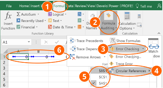
When a circular reference occurs, Excel typically displays a warning prompt immediately, and the bottom status bar will explicitly list the exact cell address causing the loop. To track down and destroy the loop, navigate to the Formulas tab on the main ribbon and locate the Formula Auditing section. Click the small arrow next to Error Checking and select Circular References from the dropdown menu. This tool will display a list of every cell trapped in the paradox. You must manually select the identified cell and rewrite its formula so that its reference range strictly excludes its own location, instantly restoring normal mathematical processing to your spreadsheet.